Marc's Notes

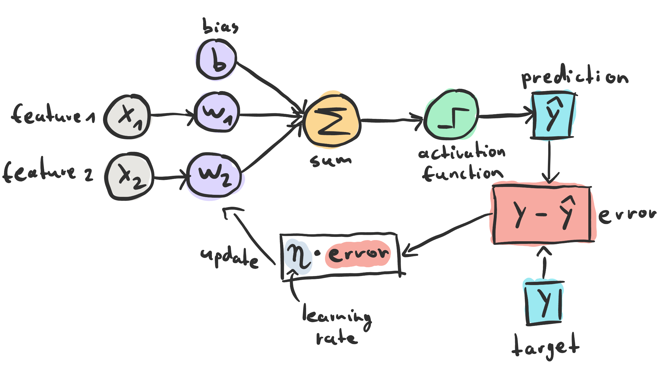
We'll be implementing a simple perceptron model for binary classification tasks using Python, and discussing the fundamentals of the perceptron model, including how it makes predictions and updates its weights during training.

The first step in implementing a simple perceptron model is to define a class that contains the weights, training loop, and prediction methods.

class Perceptron:

    def __init__(self, lr=0.01, epochs=50):
        self.lr = lr 
        self.epochs = epochs 
        self.init_weights() # TODO

Here, we already set default values for hyperparameters like the learning rate (lr) and the number of epochs that the model should be trained for. Additionally, we already initialize the weight and bias values with the init_weights method.

Weight & Bias Initialization

To initialize the weights and bias, we can either use constant values like 0 and 1, or we can choose random numbers. Since our training data has two features, we need one weight per feature, so we use two random values for the weights here.

def init_weights(self):
    self.weights = torch.rand(2) 
    self.bias = torch.rand(1)

Training Loop

Now we are ready to work on the training loop. The basic idea is that we start predicting classes with random weight values in the model. We then compare the predicted (probably misclassified) class label with the expected class label to compute the error that the model has made. We then use the error to update the weights and bias by a small amount to get better predictions. We iterate over this process until the model converges or we reach the maximum epoch limit.

At each learning step (epoch), we loop through the entire data set and update the weights and bias by a small delta value.

In the code, we can use two loops to iteratively update the values.

def fit(self, X, y):
    for epoch in range(self.epochs):
        # for every data point and label
        for xi, yi in zip(X, y):
            weight_delta = ... # TODO 
            bias_delta = ... # TODO 

            # Update weigths
            self.weights += self.weight_delta 
            self.bias += self.bias_delta

Of course, the important part is calculating the correct delta values.

The current error of the model

can take different values depending on the predictions. If the true and predicted classes are the same (0,0 or 1,1), the error will be equal to 0. In this case, everything is fine and we don't need to update the weights. In the two cases of misclassification (0,1 or 1,0), the error will be either -1 or 1. Here we want to update the weights to hopefully get the prediction closer to the correct class in the next epoch.

As you can see from the formula below, we update the weight with respect to the actual data points. This way, our data has an influence on the weight updates. Large values will have a higher impact than small values. This implies that our model benefits from feature scaling. One of the methods that could be applied is standardization where you subtract the mean and divide by the standard deviation to center and scale your data points.

We multiply by the learning rate to make smaller steps, which helps to get better convergence. The magnitude of the learning rate plays an essential role. Too large values will lead to rapid but unstable convergence, too low values will make the model converge slowly and it may even get stuck in local minima.

def fit(self, X, y):
    for epoch in range(self.epochs):
        for xi, yi in zip(X, y):
            # Compute the error and weight updates
            error = yi - self.predict(xi) # TODO
            weight_delta = self.lr * error * xi  
            bias_delta = self.lr * error

            self.weights += self.weight_delta 
            self.bias += self.bias_delta

Finally, we have to implement the predict method to be able to calculate the error.

Prediction

For prediction, we simply compute a linear combination of the input data using the trained weights and bias. To get the corresponding class labels, we need to clip the values with a step function. This gives us a binary output, just like the target variable.

def predict(self, X):
    output = X @ self.weights + self.bias
    # Activation Function (in this case a simple step function)
    pred = torch.where(output >= 0.0, 1, 0) 
    return pred

Using the Perceptron Model

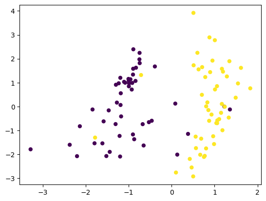
To use the perceptron model, we first need to create some sample data using the scikit-learns make_classification function. The resulting synthetic data set has two classes with two features.

X_train, y_train = make_classification(n_samples=100, n_features=2, n_informative=2, n_redundant=0, random_state=40)

plt.scatter(X_train[:,0], X_train[:,1], marker='o', c=y_train, s=25)
plt.show()

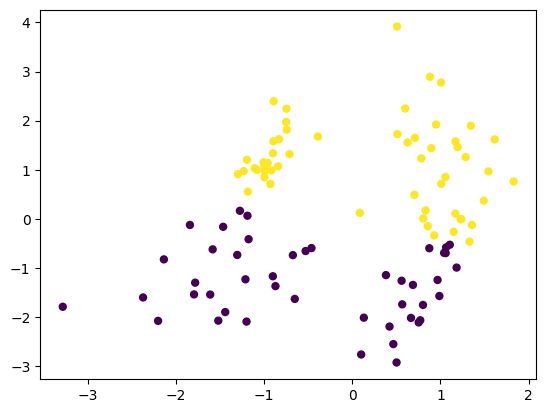
Prediction with Random Weights

First, we create a perceptron instance and predict classes without training the model.

perceptron = Perceptron(lr=0.01, epochs=100)
y_pred = perceptron.predict(X_train)

plt.scatter(X_train[:,0], X_train[:,1], marker='o', c=y_pred, s=25)
plt.show()

We can see that the random weights did not do a good job of separating the two classes.

Prediction with Trained Weights

Now, let us fit the perceptron and see whether the results are any better.

perceptron.fit(X_train, y_train)
y_pred = perceptron.predict(X_train)

Here we can see two different plots for the predictions. The left one did not use any activation function and therefore shows the full range of values that were predicted. On the right side, the step function from above was used.

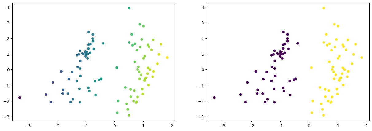
After training, the model seems to be able to discriminate between the two classes quite well. However, when comparing the predictions with the original data set we can clearly see that some samples were still misclassified. This is expected because the perceptron model is trying to fit a linear decision boundary while the two classes are actually not linearly separable. We could solve this problem by introducing more features, since in a higher dimensional space there may be a hyperplane that perfectly separates the classes. Of course, this will not always be possible which is why we need more complex models that can fit nonlinear decision boundaries.

Code

You can find the complete code here and on GitHub.

import torch
import matplotlib.pyplot as plt
from sklearn.datasets import make_classification


class Perceptron:

    def __init__(self, lr=0.01, epochs=50):
        self.lr = lr
        self.epochs = epochs
        self.init_weights()

    def init_weights(self):
        self.weights = torch.rand(2)
        self.bias = torch.Tensor([0])

    def fit(self, X, y):
        X = torch.Tensor(X)
        y = torch.Tensor(y)
        for epoch in range(self.epochs):
            total_error = 0
            for xi, yi in zip(X, y):
                y_pred = self.predict(xi)
                error = yi - y_pred
                self.weights += self.lr * error * xi
                self.bias += self.lr * error
                total_error += error
            if epoch % 10 == 0:
                print(f'epoch {epoch} \t error {total_error}')

    def predict(self, X, activation=True):
        X = torch.Tensor(X)
        output = X @ self.weights + self.bias
        if activation:
            output = torch.where(output >= 0.0, 1, 0)
        return output

perceptron = Perceptron(lr=0.01, epochs=200)
perceptron.fit(X_train, y_train)
y_pred = perceptron.predict(X_train)